Saturday, November 26, 2022

A primer on income inequality (including links to Emanuel Saez lectures)

I would like to bring to the attention of IB Higher and Standard Level Economics students as well as colleagues an article by Max Roser and Esteban Ortiz-Ospina in Our World in Data with tons of useful information for all of us, titled Income Inequality 

 
Most sections include data that can be used to incorporate in part (b), paper 1, essays that relate to income distribution.

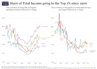
A section in this site of particular interest to IB Economics candidates is titled 'How has inequality in high-income countries evolved over the last century'

Here we see that income concentration in the US and other other English-speaking countries follows a U-shaped long-term trend.  But...

...in equally rich European countries, as well as in Japan, the development is in fact quite different. The income share of the rich has decreased over many decades, and just like in the English-speaking countries, it reached a low point in the 1970s. In contrast to the English-speaking countries, however, top income shares have not returned to earlier high levels; they have instead remained flat or increased only modestly. The evolution of top income inequality followed an L-shape here. Income inequality in Europe and Japan is much lower today than it was at the beginning of the 20th century.


On the 'U- shaped path of income concentration in the US it is also worth watching a 6 minutes Stanford University video featuring Emanuel Saez of Berkeley, one of the most important researchers of income inequality. In this short video, he provides excellent data and visuals on the fall and subsequent rise in income inequality in the US over the past 100 years.  It can be found here: The Takeoff in Income Inequality: Emmanuel Saez

A longer (16 minutes, Berkeley lecture - teach-in) version can be found here (I show it to my HL class every year): Economic Inequality Teach In: Emmanuel Saez .  

Back now to the 'Our World in Data: Income Inequality' article by Roser and Ortiz-Ospina.  The following are also sections that are all worth exploring:

  • High-income countries tend to have lower inequality
  • Top income shares 
  • Inequality in the US has been growing substantially in recent decades 
  • Inequality in different world regions 
  • Relative poverty 
  • How are the incomes of the rich changing relative to the incomes of the poor? 
  • How does income inequality differ from consumption inequality?

In my opinion, income inequality (as well as wealth inequality and inequality of opportunity) topics are a must for a well prepared IB Economics candidate.  Hopefully the above can provide some useful background information that will help students prepare for May & November exams.  

Rising inequality in our world is of course way more important than exam preparation... 


On growth

 
I have been planning to upload a post about an excellent article published by Chatham House since early October (and it is the end of November..,).  No excuses, just apologies.


The article seems dated (it focuses on Truss' 'mini budget'...) but in reality it is not at all.  It is excellent  for IB Economics students (both HL and SL).  It is why growth, the size of the pie, may not matter as much as the distribution of the pie and why focusing on growth rates may divert our attention from other more important metrics of our collective well-being and may be terribly misleading.  

This paragraph is revealing:

Looking at GDP growth alone, a highly unequal society, which is polluting and depleting its natural assets can – at least in the short-term – appear a success story. In fact, once GDP growth is accepted as a good thing in itself, it can be used to support other political agendas and interests. Faith in the ‘rising tide lifts all boats’ theory of growth can sugar-coat policies that marginalize other important elements of economic health such as fairness and resilience to shocks.

This short article is packed with links.  Many of these will help students increase the stock of real world examples they need to effectively discuss or evaluate in Paper 1, part (b), essays.  All these links of course will help them appreciate the importance of this course no matter what they plan to study later in college. One of the most interesting links directed me to the Wellbeing Economy Governments site.

The article is titled  'Why it is time to change the narrative around growth' and can be found here.

Wednesday, October 26, 2022

Some notes to my IB Economics students on the MULTIPLIER EFFECT

 THE MULTIPLIER EFFECT

A (Keynesian) idea whereby an increase in government expenditures G will lead to a greater increase in national income (in real GDP)

i.e. ΔY > ΔG or, ΔY = κ ΔG

(where little κ is the multiplier)

Let the government increase government expenditures by $100mil. If national income increases by $300mil, the multiplier (little κ) is ‘3’: $300m/ = 3 x $100m

 Why should we expect this to be the case? Because:

  • Your spending is my income.
  • Economic activity takes place in successive rounds (as clearly illustrated by the ‘circular flow of income’ diagram; use in an essay if you consider it necessary)

If the government spends $100 to build a tiny road in my neighborhood and I’m the only worker / engineer, it means that my income increases by $100.

Part of this additional income earned, I will spend on domestic goods and services, say $80. For example, from the additional $100 I earned, I will spend $80 for a dancing company to come at my birthday party and dance for my guests. National income will have increased by $100 + $80 = $180 (and note that two ‘goods’ will have been produced: a tiny road and a dancing performance).

Generalizing: If out of each dollar earned as additional income people spend 80 cents then the so-called Marginal Propensity to Consume (MPC) is 0.80

MPC = ΔC / ΔY, equal to say ‘b’

Let the dancers now spend 0.8 of their additional income on violin lessons for their offspring.  They thus spend $64 (0.8x80) on the violin teachers.  Violin teachers now have additional income equal to $64 and national income has increased by a total of $100+$80+$64 = $244.  They in turn will spend part (0.8) of their additional income on feta cheese…and so on and so forth…

More generally (a geometric series; sum of; converges as 0 < b < 1):

ΔY = ΔG + bΔG + b^2ΔG + b^3ΔG + …

ΔY = (1+b+b^2 +b^3 +b^4 +…) x ΔG

ΔY = (1/(1-b)) x ΔG, so little κ:

κ = {1 / (1-MPCd)] = {1/(MPW)], where MPW = MPS + MPT + MPM

(as if I spend out of $100 of additional income on domestic goods, the rest (i.e. $20) I have either saved (S) or paid in taxes (T) or spent, but on imports M): all three (S,T, M are withdrawals / leakages from the circular flow)

(MPS is the marginal propensity to save, MPT is the marginal tax rate and MPM is the marginal propensity to spend on imports: their sum [MPS+MPT+MPM] is the marginal propensity to withdraw : So (1-MPCd) = MPW (remember the circular flow again)  

Note:

  • The multiplier effect holds if any of the 3 injections increases (remember that injections 'J' include government expenditures G, but also exports X and private investment I) (note that the export multiplier is responsible for the international transmission of the business cycle)
  • The importance of the Keynesian multiplier of government expenditures (G) is that it shows that expansionary fiscal policy in the form of increased government expenditures (G) is very powerful to help an economy grow - lift an economy out of a recession (but, remember the other side, the crowding-out effect)
  • Expansionary fiscal is not only a result of an increase in G but could also be a result of a decrease in direct taxes T.

But, the multiplier effect of an equal (to ΔG) decrease in taxes T is smaller. Why?

Because the first-round effect does not exist. When a government decreases my taxes by $100, my income does not rise by $100: it is my disposable income that rises by $100 so the multiplier process starts with the 2nd round effect of an equal increase in G (since I will spend $80 of this increase in my disposable income on the dancing company above). So, the tax multiplier will be [b/(1-b)]  (the first term of the geometric series is now ‘b’, not ‘1’) It follows that if b is 0.8, then the government expenditure multiplier will be 1 / 0.2 = 5 but the tax multiplier will be 0.8 / 0.2 = 4 (smaller)

  • The multiplier operates also in the opposite direction. A decrease in government expenditures (G) will lead to a greater decrease in national income (Y). When Greece was ‘forced’ to borrow to avoid default during the Greek debt crisis, it ‘agreed’ to decrease government expenditures (G) as part of the agreement.  The IMF had then estimated that the Greek government expenditure multiplier, was, say equal to  ‘2’, so that a decrease in Greek government expenditures (G) by, say, €200mil., was expected to lead to a decrease of Greece’s national income by €400mil. (2x200)

BUT the recession that ensued (the decrease in national income) proved much more severe than expected: Greece’s rGDP decreased by much more than estimated by the IMF, say, by €500 million, and consequently even more people lost their jobs and their income, forcing the IMF (and its then Chief Economist, Olivier Blanchard - now at PIIE), to issue what was referred to as a “mea culpa”: a new IMF paper re-estimated ‘correctly’ the Greek little ‘κ’.

[Please check the Study Guide for other Real World Examples of the multiplier for use in part (b) of a Paper 1 essay]

Endnote:

In Keynes' General Theory we read (p. 128, Palgrave 2007 edition):

"If the Treasury were to fill old bottles with banknotes, bury them at suitable depths in disused coal mines which are then filled up to the surface with town rubbish, and leave to the private enterprise...to dig the notes up again...there need be no more unemployment and, with the help of the repercussions, the real income of the community...would probably become a good deal greater than it is."

Friday, October 14, 2022

National (Public) Debt - some notes: perhaps useful for IB Economics students

 Another 'new kid on the block' for IB Economics students (new syllabus)

What is the national (public) debt?

It refers to what a government owes to all of its lenders: ‘Public debt is created through government borrowing from individuals, corporations, institutions, and other governments’ [from the New Palgrave Dictionary of Economics]

è Debt is created when a government records a ‘budget deficit’: when G > T (when government expenditures exceed government income which is mostly tax revenues (T) but may also be any one-off proceeds from privatizations (the transfer [=sale] of state-owned assets to the private sector) and any profits from state-owned enterprises)

è It follows that the public debt is the sum of all past budget deficits minus any budget surpluses [‘the public debt a stock at any given point in time and represents the net accumulation of the associated deficits over all previous time periods’; from the New Palgrave]

è Given that a government borrows by issuing bonds  (=selling to whoever is willing to buy these i.e. to lenders) it follows also that the debt is equal to the value of all outstanding bonds (i.e. bonds that are held by its creditors and thus have not yet ‘matured’ and been paid off)

è Government bonds may be held by domestic creditors (=lenders) or by foreigners (= external debt; denominated typically but not necessarily in USD); bonds are held by individuals, firms, banks, universities, pension funds, money managers etc. etc.

To compare the size of the debt of a country with other countries or to determine the extent to which it is ‘sustainable’ , the absolute ‘dollar’ size of the debt is expressed as a proportion of GDP (scaling for the size of the economy).  We thus focus on the debt to GDP ratio.

(perhaps subscribe for free to Finance & Development, an IMF publication; the IMF will send you at your address every quarter the newest issue: https://www.imf.org/en/Publications/fandd

Perhaps read read: (a) https://www.imf.org/en/Publications/fandd/issues/2022/03/Balancing-act-Gaspar (b) https://www.imf.org/en/Publications/fandd/issues/2022/03/Deciding-when-debt-becomes-unsafe-Blanchard

Perhaps also check out the post on Jason Furman here: http://www.ibeconomics.org/2021/09/the-national-debt-expressed-as.html

Note:

A more appropriate metric of debt is the ‘debt service over GDP’.  The reason is that debt is a ‘stock’ variable (measured at a point in time, (say, December 31st of the year) whereas GDP is a ‘flow variable’ (measured over a time period, typically over a year).  If Janice earns income of $100000 per year and has borrowed to buy a house $300000 dollars (so owes banks $300000 (her debt)),  then her debt to her income ratio is 300000/100000 or 300% of her income - but if she needs $10 000 per year to service her debt then the debt service to her income ratio is 20% and what matters to Janice is what she pays off annually to her creditor (the bank).  That is why the debt service to GDP ratio is more informative than the simple debt to GDP ratio.

Cost of high debt 

Cost of debt servicing: 

-      a. Opportunity cost of the funds sacrificed as these funds could have been invested by the government in pro-growth and pro-development goals i.e. on infrastructure investments, on education and on health care services; debt servicing thus restricts the ‘discretionary spending’ ability of the government

-      b. Policymakers cannot as easily adopt expansionary fiscal policy (G up; and/or T down) since It would lead to more debt accumulating

-      c. If debt is mostly domestically held (as it is in Japan) and if the country (unlike Greece- a member of the Eurozone) can issue its own currency, then, if debt is getting dangerously high, the government may be tempted to ‘monetize’ its debt i.e. to print more money to pay off its creditor; but then there is higher risk of inflation (remember Friedman’s helicopter money drop: ‘too much money chasing after too few goods’); on the other hand, if an attempt is made to pay off foreign lenders (in USD) by printing more domestic currency then the currency will massively depreciate also creating higher inflation as prices of imported goods will rise.

·        Impact on credit rating:

Credit rating agencies (CRAs) measure the credit risk of debt for all types of investors. 'Their measurement of credit risk includes default probabilities…and serve an economic purpose as they reduce asymmetric information about issuers that investors face when making investments’(from the New Palgrave). Three agencies (Moody’s, Finch, Standard & Poor’s: the ‘big three’) rate the debt of countries and assign a ‘grade’.  Top rated debt (bonds) is AAA which means ultra-safe: creditors will definitely get their money back. But if these agencies come to a realization that a country’s debt is becoming riskier then it will downgrade it. But then lenders will demand a ‘risk premium’ i.e. to earn higher interest rates. This automatically makes the debt burden heavier so a ‘feedback loop’ may be initiated that may lead to default  [and here comes the IMF with its rescue packages (conditional lending at preferential interest rates) that (once 'agreed' upon) hopefully signal to private investors that the country is back on track to become creditworthy].

·        Impact on future taxation and government spending:

This is where ‘austerity policies’ come into play: the debtor country is forced (‘agrees’= more like some ‘arm twisting’) to slash G and to raise T in order to achieve ‘primary budget surpluses’ (a primary budget surplus is recorded when government spending excluding debt servicing is less than government income (T) so that the government can start lowering its debt; Greece was required for a number of years to achieve primary budget surpluses equal to 3% of its GDP which were huge and inflicted significant pain on mostly low income Greek households

-      Note an influential paper by Alberto Alesina and Silvia Ardagna that tried to show that fiscal contraction will not have the expected Keynesian result (to lead to recession) but will lead to expansion (referred to as ‘expansionary fiscal contraction’); Why? Because according to A&A the private sector would see that the government is rationalizing (cutting) its spending that would result in greater confidence levels and thus more investment and consumption from the private sector. Proved to not really be the case. Krugman called this the ‘confidence fairy’)(see https://www.bruegel.org/blog-post/expansionary-fiscal-contractions-and-uk-experiment)

-      Also note paper by Kenneth Rogoff and Carmen Reihhart of Harvard that showed that when the debt to GDP level exceeds 90% then an economy will fall into recession. A graduate student at UMass @Amherst trying as an exercise in econometrics to duplicate their results couldn’t. He and his advisor found that R&R had (a) excluded from their sample countries which if they were included would NOT have led to recession but to continued growth and (b) that there were coding ‘errors’ in their excel files. Paper was largely discredited but it had already damaged many in debt-ridden economies.

-      The ‘mea culpa’ of the IMF:  The IMF had underestimated the Greek multiplier so that the agreed upon cut in Government expenditures  by the Greek government led to a much bigger than projected decrease in national income (which meant that many more than expected suffered a loss in jobs/ income). Olivier Blanchard, then Chief Economist at the Fund (now at PIIE), was forced to issue a correction of the multiplier which was referred to as Blanchard’s ‘mea culpa’.


Monday, October 10, 2022

The notes to my IB economics (HL) on the Phillips Curve

For whatever they're worth I am posting here the notes that I have prepared for my students on the Phillips Curve.  

The Phillips Curve (notes by CZ - The IB at Athens College [901])

1958:  A.W. Phillips (LSE) published an empirical paper:

He collected annual UK data on the rate of unemployment and the percentage change in money wages for 96 years: 1861 – 1957 (money wage: whatever is written on your paycheck)

He noticed an inverse relationship between the annual percentage change in money wages and the annual UK unemployment rate: years when UK unemployment was low (= ‘tight’ labor), money wages increased significantly whereas years when unemployment was high (=’slack’ labor market), money wages increased by a little or not at all (compared to the previous year) or may even had decreased.

BUT:

·        If the wage bill for firms represents a big chunk of their total production costs

·        And, if prices are set by firms as a ‘markup’ on unit costs (i.e. say, 10% or 50% more than the average cost of producing, say, ‘pencils’)

THEN, if money wages rise a lot, prices will rise a lot (i.e. inflation accelerates) and if money wages increase a little (or, decrease) then inflation will be lower (i.e. disinflation)

Thinking along these lines many economists (Samuelson, Lipsey et al.) checked for many countries & for different time periods the data on the behavior between the annual rate of inflation and the rate of unemployment. And, OMG, they found that in many countries over many periods of time an inverse (=negative) relationship existed between inflation and unemployment: if unemployment was decreasing, inflation was increasing and if inflation was decreasing, unemployment was increasing.

This inverse relationship between the annual rate of inflation and the rate of unemployment is referred to as the (original) Phillips curve.


This empirical relationship was fully compatible with the ruling at the time Keynesian theory (remember that in the Keynesian model the level of equilibrium real output - of economic activity - is 'demand-driven': it is ‘effective’ (aggregate for us) demand that determines the level of economic activity [the equilibrium real output]):


If AD rises (from AD1 to AD2), then real GDP rises (from Y1 to Y2) so unemployment falls but inflation increases (APL1 to APL2); if AD decreases (from AD1 to AD3) then unemployment rises but inflation decreases (APL1 to APL3).

The original PC illustrated a trade-off between inflation and unemployment and if this relationship is stable through time for a country, then it was as if it presented policymakers a ‘menu of choices’: they could choose that combination on the country’s Phillips Curve that was considered the most desirable.

They could choose and achieve the desired combination using demand-side policies (fiscal (i.e. ΔG, ΔT) and monetary (i.e. Δr).

They even thought back then that they could ‘fine-tune’ the economy (which was of course considered by many as ‘hubris’).

BUT, in the early 1970s this ‘stable’ relationship between the rate of inflation and the rate of unemployment of a country collapsed.

Economies started witnessing something that was incompatible with the Keynesian model: BOTH the rate of inflation AND the rate of unemployment were increasing!  It was as if the Phillips Curve was shifting outwards (to the right).

This phenomenon was referred to as stagflation (=stagnation + inflation).

Arthur Okun (Okun’s Law: a 1% decrease in real GNP growth was associated with a 0.3% increase in unemployment) back then devised his Economic Discomfort Index — which Ronald Reagan renamed the Misery Index — the sum of the unemployment rate and the inflation rate. 

This collapse was the result of the 1st oil crisis, as in 1973, OPEC to ‘punish’ the West  for supporting Israel, restricted the supply of oil and thus quadrupled overnight the price of a barrel of oil (think now of the price of natural gas surging given that Russia is restricting natural gas exports and its impact on European and other economies).

We now realize (with our  current AD and AS tools) that because production costs increased across the board, the SRAS decreased and shifted left leading to higher inflation AND higher unemployment.

MOST IMPORTANTLY, in 1968, Milton Friedman (the most renowned Monetarist; Nobel prize) published a most influential paper titled “The Role of Monetary Policy” where he introduced the term Natural Rate of Unemployment (NRU).

His analysis of the Phillips Curve relationship distinguished between the ‘short run’ and the ‘long run’ (Remember: short run when only some, but not all adjustments are possible; long run is when all adjustments are possible)

·        He claimed that if there is a trade-off between the 2 variables it exists ONLY in the short run; in the long run, there is only one rate of unemployment, the natural rate, which is compatible with ANY rate of inflation as long as this rate of inflation does not change (does not accelerate).  Thus, in the long run the Phillips Curve according to Friedman is VERTICAL at the NRU.

·        He included in his analysis ‘expectations’ about next year’s inflation that workers form à the ‘expectations-augmented Phillips Curve’ or, the “Phelps-Friedman Critique’ {Ed Phelps came up with pretty much the same analysis independently}

·        Friedman claimed that workers form their expectations ‘adaptively’: they form their expectations about next year’s inflation by looking at last year’s inflation (‘backward’ looking expectations) (really, a weighted average of previous rates)

·        Workers thus suffer from “money illusion” i.e. they do not realize immediately that their real wage (the purchasing power of their money wage) decreased when inflation accelerated à their expectations of inflation are slow to adjust (‘adaptive’)

·        If the government tries to lower unemployment below the NRU using expansionary fiscal (and perhaps easy monetary), inflation will accelerate and workers will not immediately realize that inflation is higher than expected and thus their real wage has decreased: they will thus accept jobs offered by businesses who face lower real costs à unemployment does fall but inflation is now higher.


 When expectations of inflation adjust (long run) so that expected inflation equals actual inflation, workers will demand higher money wages (remember that money wages are flexible fully adjust to changes in the APL in the monetarist model) until the real wage is ‘restored’ back to its original equilibrium level so that in the long run, unemployment will return to its natural rate BUT with higher inflation (this analysis is the ‘mirror image’ of the AD/SRAS/LRAS model explaining how an inflationary gap is closed in the Monetarist model – see the SG)

·        To maintain thus unemployment below the NRU with expansionary demand side policies a government would have to engineer ever accelerating inflation, which of course does not make much sense.

·        Friedman’s policy recommendation is thus: “Ms. Policymaker, do not try to lower unemployment below the NRU using expansionary policies; if you are successful, your success only will be short-lived (temporary) because workers’ expectations of inflation will [eventually] adjust and thus unemployment will return to its NRU but with higher inflation”

·        Friedman quoted Abraham Lincoln that ‘you can fool some of the people all of the time, all of the people some of the time BUT NOT all of the people, all of the time”. 

      Remember:  Short run: when actual inflation exceeds expected inflation 

         Long run: when expectations of inflation have adjusted so that expected inflation is equal to actual inflation. 

       Note that now in a part (a) essay asking to explain the NRU we now have three points to explain:

1. It is the unemployment that exists when the economy is at its potential level of real output

2. It is the unemployment that exists when the labor market is in equilibrium (see in the OUP Study Guide p. 92 the Dornbusch & Fisher LD/AJ/LF labor market diagram with the real wage on the vertical) 

3. From the above analysis we now realize that the NRU is the lowest unemployment that can be achieved without inflation accelerating (NAIRU=non-accelerating inflation rate of unemployment)

Also note that unemployment in the US after the 2009 crisis was continuously decreasing: it reached 5%, then 4.5%, then 4.3%, then 4.0% then 3.8% without inflation accelerating.

So many economists as unemployment was decreasing were afraid that if the Fed did not hit soon enough the brakes (i.e. start tightening monetary policy i.e. raising ‘r’), inflation would start showing its ugly face.

Janet Yellen, who was then the Chair of the Fed, resisted these calls and kept interest rates very low (continuing ‘quantitative easing’) à unemployment thus continued to fall, reaching a 50-year record low at 3.5% WITHOUT inflation exceeding the 2% target.[BTW, Yellen's successor, Ben Bernanke, today shared with two other economists the 2022 Nobel Prize in Economics]

Thus, thousands of American households found a job à if the Fed had tightened earlier, as several economists and politicians were insisting, many poor US households would have remained unemployed (on the other hand, quantitative easing [QE] increased income inequality as explained elsewhere)

Back then, many economists had started wondering whether the PC is ‘dead’, whether it was ‘hibernating’, why has it ‘flattened’ etc.

Explanations for the observed phenomenon varied. A couple of accessible to IB Higher Level Economics students include: 

a.   Discouraged workers re-entering the labor market and finding jobs so that U, the numerator, in the unemployment statistic didn’t rise but the labor force number (the denominator) increased, decreasing the rate of unemployment {w/o need for firms to raise wages and thus prices to attract workers}.

b.   Expectations of inflation back then were well ‘anchored’ at the 2% target rate so that neither firms felt the need to raise prices, nor did workers feel the need to demand higher money wages: all stakeholders expected inflation to remain at 2%.

This explains why NOW, the Fed and analysts fear that inflationary expectations are ‘unmoored’ (=de-anchored) which, if true, implies that US inflation will continue to rise. A Central Bank must be credible – which is why Powell (the Chair of the US Fed) sounds so firm about the Fed’s intentions.  [many claim and they seem to be right that the Fed should have tightened monetary policy earlier - it was 'behind the curve']

PLEASE watch Aspen’s Roundtable on the US Economy and pay close attention to what exactly Neel Kashkari (President of the Federal Reserve Bank of Minneapolis) says: 

http://www.ibeconomics.org/2022/08/a-most-interesting-roundtable-organized.html


Monday, August 15, 2022

The End of Magic Money


In the July 2022 issue of Foreign Affairs there is an interesting article titled "The End of Magic Money: Inflation And The Future Of Economic Stimulus". In it the author explains how, "under the right conditions, magic money can undoubtedly be deployed successfully" and how US policymakers were successful in dealing with the 2008 financial crisis and how the first response to Covid-19 was also impressive. 

"The pandemic caused U.S. GDP to collapse in the second quarter of 2020: output shrank at an annualized rate of 32 percent. This fall was four times deeper than the hit from the financial crisis in the fourth quarter of 2008; indeed, it was the sharpest ever contraction in the post–World War II period. The Fed responded aggressively, creating twice as much money as it had from 2008 to 2009. Likewise, the president and Congress delivered a budget stimulus that was twice as big as the 2009 version."

This 'mega-stimulus' worked perfectly as the economy 'bounced back' to pre-pandemic levels 'with no sign of inflation' writing that "If the authorities had been able to stop there, they would have pulled off a textbook example of macroeconomic stabilization".

 According to the author, Sebastian Mallaby, "Starting in the spring and summer of 2021, the Fed committed three mistakes, opening the door to today’s price surge".  As a result of the March 2021 $1.9 trillion fiscal stimulus, Brookings forecast that by the end of 2021 the US economy 'would be operating above its maximum sustainable level'. All IB economics students should precisely understand what exactly this implies.  That was the first error according to Mallaby. The Fed did not tighten at that point, preferring to take a 'wait-and-see approach (which is understandable, given the uncertainty faced at that point).  For many it should have 'hiked interest rates, snuffing out the inflation before it became serious'.  Back then many academics claimed (most notably Krugman) that the rise in inflation was 'transitory' (see my earlier post on the debate between 'team transitory' and 'time persistent'; the Summers-Krugman debate, where Laurence Summers proved right: A primer on inflation).  

Then Mallaby goes on to explain the second error the Fed made.  in March 2022 it increased interest rates by only 25 basis points (0.25%), the smallest possible increase. Why? According to Mallaby it was because the Fed is "attached to 'forward-guidance', the practice of signaling interest-rate moves well ahead of implementing them". He calls this the 'speak-wait-act triple jump approach' which may be useful is inflation is too low (the ZLB problem monetary policy faces; you can check if you wish the Oxford IB Economics Study Guide volume on this: pages 98, 118, 122-123, 131, 140-142) but is not useful when the central bank faces the 'opposite challenge of high inflation'. Sometimes 'speed is the priority' when dealing with inflationary pressures arising.  

The third error relates to the fear that a sizable increase in interest rates would spook financial markets.  'Calling market tops is hard, and the Fed's caution is understandable'. But 'asset prices were screaming that the economy was running hot'.  According to Mallaby again, the Fed should have 'factored financial signals into its decisions' and tightened earlier.

The circumstances are such that 'magic money...for the foreseeable future is off the table'. Achieving price stability (the 2% average that Neel Kashkari of the Minneapolis Fed  reiterated in the Roundtable - see my post) is of paramount importance and this will perhaps be more difficult now because 'globalization has stalled' and many many economies are 'stockpiling strategic commodities and "friend-shoring" supplies which is inflationary.

The article IMO is excellent for IB Economics students as it provides them with examples of macroeconomic policies that helps their understanding and can be used in Paper 1 essays.

This is the link: The End of Magic Money Worth your time.

(if not a Foreign Affairs subscriber you can enter your email and they'll send a paywall-free link directly to your inbox).

The logic of carbon pricing

The new IB Economics syllabus expects a lot from students on
 
  • Negative externalities of production
  • Common pool resources
  • Government intervention in response to externalities and common pool resources including carbon pricing
This piece (see link below) by Max Roser published in June 2021 on carbon pricing in Our World in Data is exactly what an IB Economics candidate (HL and SL) should read to understand the logic behind it.

Quoting from the article:
Consequences include the negative economic impacts of climate change through its effects on people’s livelihoods, and the damage to infrastructure through rising sea levels, thawing permafrost, and extreme weather events. They pose a large threat to the life of animals and ecosystems on our planet and include the destruction of coral reefs, forest fires, the loss of ice shields, and the expansion of deserts. They include an increase in extreme weather events, like heat waves, droughts, floods, and storms. And especially for the world’s poorest people they pose a threat to their lives, as they increase the risk of hunger and food insecurity.

Climate change isn’t the only negative consequence of burning fossil fuels. The air pollution that is caused by burning fossil fuels kills an estimated 3.6 million people in countries around the world every year. 

This is the price we are already paying for burning fossil fuels.
 The author goes on to explain that
There are two ways in which a carbon price can be implemented: a carbon tax or a ‘cap and trade’ system:

In a ‘cap and trade’ system the carbon price changes over time. A maximum level of pollution (a ‘cap’) is defined and manufacturers need licenses to emit carbon. How expensive these licenses are is determined by a trading system. The price of a license increases as emissions approach the cap. 
A carbon tax is simply a levy that is applied to all goods and services which lead to carbon emissions in their production. 
In both systems the price of any product increases with the amount of carbon emitted in the production of it. The result is that products with a low carbon footprint (like taking the train or solar energy) do not get more expensive, while goods that do create a lot of emissions (like a flight or coal energy) do get more expensive.

This helps us reduce emissions and pollution in two ways: it makes carbon-intensive goods much more expensive, meaning consumers will opt for cheaper low-carbon alternatives when they are available; and in markets where they’re not available yet producers will be incentivised to develop low-carbon alternatives.
The link for this excellent Max Rosen article is here: The Argument for a Carbon Price


Carbon pricing can take the form of either a carbon tax or a 'cap and trade' system.  An excellent (brief and simple) article comparing the two is by Charles Frank of Brookings:
A carbon tax is one way to put a price on emissions. Cap-and-trade is another. A carbon tax and cap-and-trade are opposite sides of the same coin. A carbon tax sets the price of carbon dioxide emissions and allows the market to determine the quantity of emission reductions. Cap-and-trade sets the quantity of emissions reductions and lets the market determine the price. Which of the two is better?
Frank breaks down his simple analysis into four sections:
  • which has greater uncertainty and imposes more risks?
  • which is easier and less costly to administer?
  • which is more likely to be politically palatable?
  • what mix of policies combines the best of cap-and-trade and a carbon tax?
There are of course real world examples for students to use.
The link to this Brookings article is here: Pricing Carbon: A Carbon Tax or Cap-and-Trade

Finally, Ian Parry,  the Principal Environmental Fiscal Policy Expert at International Monetary Fund, has these has this list of Five Things to Know about Carbon Pricing for IB Economics students.  Brief and easy.

PS: Complementary to the above is of course ending fossil fuel subsidies.  Students can check out this one: greenhouse gas emissions we should not pay people to burn fossil-fuels, again by Max Roser at Our World in Data.

Hope these help IB Economics students thinking about this issue and tackling effectively related exam questions.

Nota Bene!👇

I just read an Opinion in the New York Times by Paul Krugman written on 16/8/22 and titled 'Why We Don’t Have a Carbon Tax'.  I decided to add his opinion here to help students have a (slightly) different view in related Paper 1 essay questions.  

Bottom line is that he does not  consider carbon pricing a panacea to the climate change challenge we face.  He writes about the Inflation Reduction Act that Biden in the US just signed (according to Krugman 'despite its name, [it] is mainly a climate bill') which 'relies almost entirely on subsidies intended to promote clean energy, offering tax credits for renewable energy, aid to keep nuclear plants operating, incentives to buy electric vehicles and make homes more energy efficient and more'. He continues arguing that 'an exclusive focus on carbon taxes was “dubious economics and bad political economy.'  A carbon tax would be bad political economy because 'people aren’t just consumers and taxpayers, they’re also workers. And any policy that reduces greenhouse gas emissions will displace jobs in fossil fuel industries.'  It would be interesting to point here to the objection that Larry Summers voiced in the roundtable concerning this displacement (go to 34:53) where at 35:17 he ask the rest to put this displacement issue in perspective saying that 'there are only 50000 coalminers in the United States of America right now.  That is one sixth of the number of manicurists...'! Following Krugman's arguments he concludes the piece by writing 'Does this mean that we should never impose a carbon tax? No, not at all. [But,]There’s still a good case for giving people a direct financial incentive to limit emissions, and such a thing may become politically possible as the economy decarbonizes and green energy becomes a more powerful interest group.'
This excellent (short and sweet) complementary article to the above can be reached by clicking here: 
Why we don't have a carbon tax (of course, he is referring to the US). Enjoy!

PS1: The 2019 Twitter thread Krugman refers to in the article is here 


PS2: Olivier Blanchard, the senior fellow at PIIE (also ex-chief economist at the Fund and MIT professor) another heavyweight also weighs in on the carbon tax vs green subsidies debate sparkled by IRA 'climate bill'; Blanchard argues that carbon pricing (carbon taxes) are necessary as (a) a subsidies only approach may prove way too costly for the Government (b) the effectiveness of such subsidies varies significantly and (c) carbon taxes are needed to finance such subsidies
This debate is great for IB Economics students.  The debate is now on Twitter:

Friday, August 12, 2022

A Roundtable on the US Economy to watch (easy and useful)


A most interesting roundtable organized the other day at the Aspen Institute on whether the US economy is headed towards stagflation.  

Excellent for IB HL Economics candidates.  

Exposure to what is going on in a major economy by Lawrence Summers of Harvard, Neel Kashkari of the Minneapolis Fed, Melissa Kearney Professor at the U. of Maryland and of the Aspen Economic Strategy Group and Lawrence Fink, the CEO of BlackRock that manages $10 trillion in assets.  The discussion was moderated by Greg Ip, of the WSJ and author of the great book The Little Book of Economics. Many connections with the current Economics syllabus.  


The video link is here: Is the US Headed for Stagflation


How do we measure living standards


Very often in HL and SL IB Economics exams, candidates are asked questions that relate to living standards and how can we compare across countries or through time.  The new syllabus pays even more attention to this topic so it is recommended that student research it more.

One thing to keep in mind is that even Simon Kuznets, the economist who developed national income and product accounts, warned against using per capita income as a way to make such comparisons.  

A December 2021 article by Benjamin, Cooper and Kimball, titled Measuring the Essence of the Good Life is, in my opinion at least, a must read for any serious student of IB Economics walking into May or November final exams. It was published in Finance & Development, an IMF free publication.  This publication has numerous (short!) articles that perfectly align with the requirements of our syllabus. And students (or an instructor) can request free hard copies.  Many of my students have and they thoroughly enjoy it!

The link to this interesting and useful  article is here: Measuring the Essence of the Good Life (8 minutes read)